SWIM-RS Algorithm Description¶

Overview¶

SWIM-RS (Soil Water Inverse Modeling with Remote Sensing) implements a modified FAO-56 dual crop coefficient soil water balance model driven by remote sensing observations. The model simulates daily evapotranspiration, soil moisture dynamics, irrigation, and groundwater interactions for agricultural fields. We use NDVI time series from satellite imagery to estimate crop coefficients dynamically, enabling spatially distributed ET estimation without crop-specific parameterization.

SWIM-RS includes supporting infrastructure around the core water-balance model:

Data ingestion and storage are handled by SwimContainer, which organizes the many inputs and derived datasets needed to run the model. See container architecture.
Simulation inputs and state are represented with a small set of explicit objects: SwimInput, FieldProperties, CalibrationParameters, and WaterBalanceState. See process architecture.

This modular design keeps components testable and makes it easier to extend SWIM-RS with new features (e.g., alternative snow/runoff/soil-water formulations, richer irrigation scheduling, and new remote-sensing proxies for ET and Kcb).

While this software has been completely rewritten, it was originally based on a fork of et-demands; shoutout to Dr. Richard Allen, Chris Pearson, Charles Morton, Blake Minor, Thomas Ott, Dr. Justin Huntington, and others who've contributed to that project over the years. For a detailed comparison of the two codebases, see ET-Demands Comparison.

Model Inputs¶

Meteorological Forcing¶

Reference ET (ETr or ETo): Alfalfa or grass reference evapotranspiration (mm/day)
Precipitation (prcp): Daily total precipitation (mm)
Temperature (tmin, tmax): Daily minimum and maximum air temperature (°C)
Solar radiation (srad): Incoming shortwave radiation (MJ/m²/day)

Remote Sensing Observations¶

NDVI time series: Normalized Difference Vegetation Index, interpolated to daily values

Soil Properties¶

AWC: Available water capacity (mm/m)
CN2: Curve number for average antecedent moisture condition
Ksat: Saturated hydraulic conductivity (mm/hr), used for infiltration-excess runoff
REW: Readily evaporable water in surface layer (mm)
TEW: Total evaporable water in surface layer (mm)
zr_max: Maximum root depth (m)

Management and Field Properties¶

Irrigation schedule flags: Boolean flags indicating irrigation days
Irrigation status: Whether field is irrigated
Perennial status: Whether crop has persistent root system
Groundwater status: Whether groundwater subsidy is available

Daily Iteration Structure¶

We iterate through each day in the simulation period. For each day, we perform the following calculations in sequence, updating the water balance state.

Note on step numbering: The steps below are numbered for conceptual clarity, not execution order. In the implementation (loop.py:step_day), the actual sequence differs for physical correctness:

Snow partitioning and melt (Step 2) - needed to determine effective precip
Runoff calculation (Step 3) - depends on rain vs snow
Crop coefficient from NDVI (Step 1)
Fractional cover (Step 4)
Root depth calculation (Step 5) - computed early but applied at end
TAW/RAW computation, surface layer update
Kr/Ks coefficients (Steps 6-7)
Actual ET (Step 8)
Irrigation and groundwater (Steps 9-10)
Deep percolation (Step 11)
Root growth water redistribution (Step 5 completion)

Algorithm Steps¶

Note: Many of the FAO-56 Modifications below are based on qualitative and quantitative analysis of five eddy covariance flux towers in the Western US: US-FPe (Fort Peck, MT), S2 (Crane, OR), US-Blo (Sierra Nevada, CA), MR (Muddy River, NV), and ALARC2_Smith6 (Yuma, AZ). The other hundreds of flux towers were held out of the testing process and used to assess model generalization and validation metrics.

Step 1: Basal Crop Coefficient from NDVI (FAO-56 Modification)¶

We compute the basal crop coefficient (Kcb) from NDVI using a sigmoid relationship:

Kcb = Kc_max / (1 + exp(-ndvi_k × (NDVI - ndvi_0)))

The exponent is clipped to [-20, 20] to prevent numerical overflow.

Parameter interpretation:

ndvi_0 (inflection point): The NDVI value at which Kcb = Kc_max / 2. This controls when transpiration "turns on" as vegetation develops.
ndvi_k (steepness): How sharply Kcb transitions from low to high values around the inflection point. Higher values create a more step-like response.
kc_max (ceiling): Maximum basal crop coefficient at full canopy.

Land-cover dependence of ndvi_0:

At calibration test sites, we found that optimal ndvi_0 varies substantially by vegetation type:

Land Cover	Calibrated ndvi_0	Interpretation
Grassland (US-FPe)	0.14	Sparse cover already transpires; sigmoid activates early
Irrigated alfalfa (S2)	0.58	Transpiration delayed until substantial canopy closure

This reflects phenology: grasslands transpire proportionally to any greenness, while dense crops require substantial canopy development before reaching maximum transpiration rates.

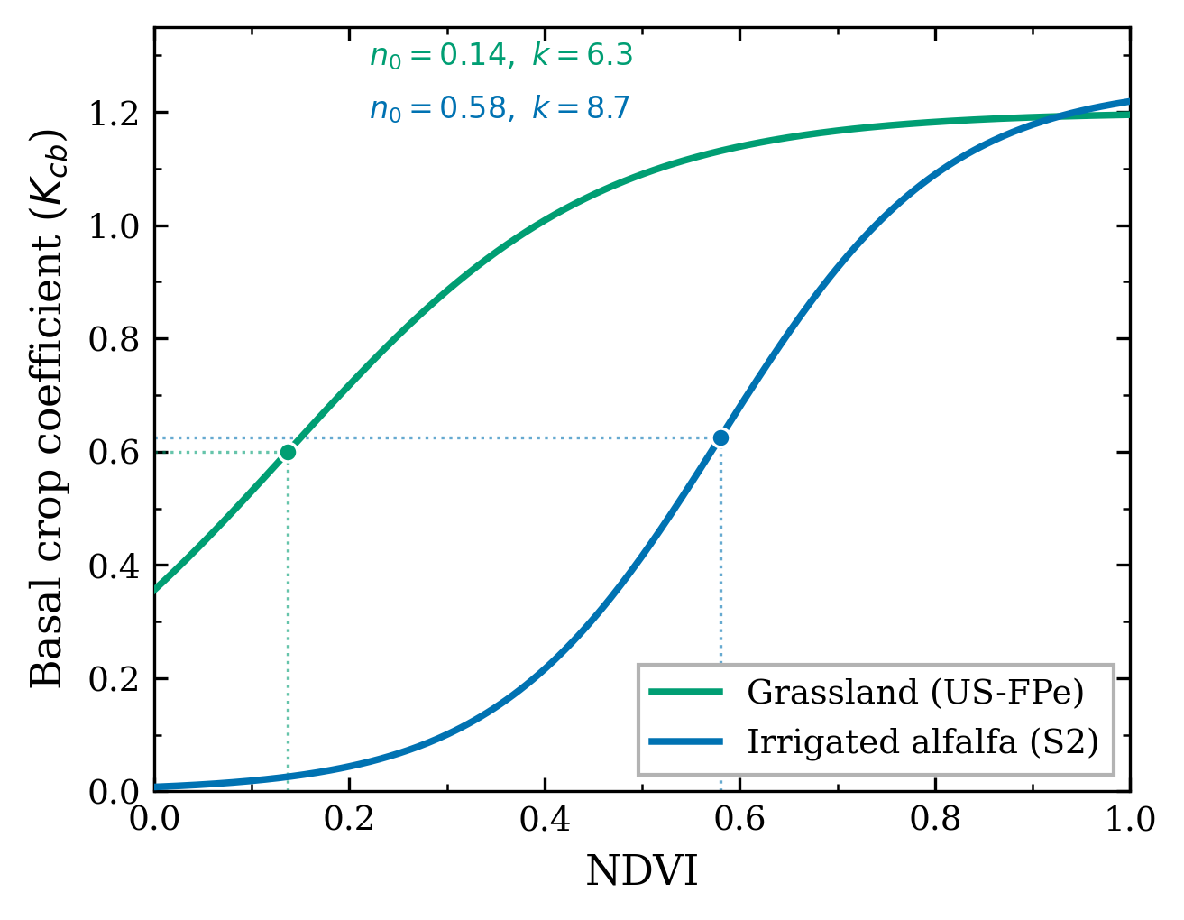
Sigmoid response curves for grassland and irrigated alfalfa

Figure 1: Calibrated NDVI→Kcb sigmoid curves for two flux tower sites. The inflection point (dot) marks where Kcb = Kc_max/2. Grassland (US-FPe) activates at low NDVI, while irrigated alfalfa (S2) requires near-full canopy.

Parameters: ndvi_k (slope), ndvi_0 (inflection point), kc_max (ceiling)

Step 2: Snow Dynamics¶

We partition precipitation into rain or snow and compute snowmelt:

Partitioning:

If T_avg < 1°C: precipitation falls as snow
If T_avg ≥ 1°C: precipitation falls as rain

Albedo evolution:

Fresh snowfall (> 3 mm) resets albedo to 0.98
Albedo decays exponentially with two rates:
- With some snowfall (0-3 mm): decay rate = 0.12
- With no snowfall: decay rate = 0.05 (slower aging)
Decay formula: albedo = albedo_min + (albedo_prev - albedo_min) × exp(-decay_rate)
Minimum albedo for old snow: 0.45

Snowmelt (combined degree-day and radiation approach):

melt = (1 - albedo) × srad × swe_alpha + max(T_avg - 1.8, 0) × swe_beta

Melt is bounded by available SWE
No melt occurs when T_max ≤ 0°C

Parameters: swe_alpha (radiation melt coefficient), swe_beta (degree-day factor)

Step 3: Runoff Calculation¶

Two methods are available, selected via runoff_process:

Curve Number (CN) Method (runoff_process = "cn"):

We adjust CN for antecedent moisture based on surface layer depletion:

Wet conditions (low depletion): CN → CN_III (higher runoff)
Dry conditions (high depletion): CN → CN_I (lower runoff)

Runoff is calculated using the SCS equation:

S = 250 × (100/CN - 1)
Ia = 0.2 × S
Q = (P - Ia)² / (P - Ia + S)  when P > Ia

For irrigated fields, we smooth runoff using a 4-day average of S values to reduce irrigation-induced variability.

Infiltration-Excess Method (runoff_process = "ier"):

Uses hourly precipitation vs. infiltration capacity:

Q = Σ max(P_hr - Ksat_hr, 0)

Infiltrating precipitation = rain + snowmelt - runoff

Step 4: Fractional Cover and Exposed Soil¶

We compute fractional vegetation cover from Kcb:

fc = (Kcb - Kc_min) / (Kc_max - Kc_min)
few = 1 - fc

fc is bounded [0, 0.99] to ensure exposed soil fraction remains positive
few is bounded [0.01, 1.0] for numerical stability
few represents the fraction of soil available for evaporation

Step 5: Root Growth¶

For annual crops, root depth varies with crop vigor:

zr = zr_min + (zr_max - zr_min) × (Kcb - Kc_min) / (Kc_max - Kc_min)

For perennial crops, root depth remains constant at zr_max.

When roots grow or shrink, we redistribute water between the root zone and layer 3 to conserve mass.

Step 6: Surface Evaporation (Kr and Ke; FAO-56 Modification)¶

Evaporation reduction coefficient (Kr):

Kr = (TEW - De) / (TEW - REW)  when De > REW
Kr = 1                          when De ≤ REW

We apply damping to smooth day-to-day transitions:

Kr_new = Kr_prev + kr_damp × (Kr_current - Kr_prev)

This is a simple “inertia” term: each day, Kr moves a fraction kr_damp of the way from its previous value toward the current value implied by surface wetness. Increasing kr_damp makes evaporation respond more quickly to wetting and drying (sharper post-rain Ke pulses), while decreasing kr_damp makes the response slower and more memory dominated.

Evaporation coefficient (Ke):

Ke = min(Kr × (Kc_max - Kcb), few × Kc_max)
Ke = min(Ke, Ke_max)

The dual constraint ensures evaporation doesn't exceed available energy or exposed soil area.

Parameters: kr_damp (damping factor), ke_max (maximum soil evaporation)

Step 7: Root Zone Stress Coefficient (Ks; FAO-56 Modification)¶

When root zone depletion exceeds RAW, transpiration stress begins:

Ks = (TAW - Dr) / (TAW - RAW)  when Dr > RAW
Ks = 1                          when Dr ≤ RAW

Where:

TAW = AWC × zr (total available water)
RAW = MAD × TAW (readily available water)
MAD is the management allowed depletion fraction

Note on MAD in SWIM-RS (parameter overloading): In FAO-56, MAD (denoted p) primarily defines the stress onset threshold (RAW) used to compute Ks. In SWIM-RS, the same RAW threshold is also reused to trigger irrigation and groundwater subsidy (both check Dr > RAW), so calibrated MAD is best interpreted as a tuned control/stress threshold rather than a directly measured management depletion fraction.

We apply damping for smooth response:

Ks_new = Ks_prev + ks_damp × (Ks_current - Ks_prev)

This damping has the same intuition as Kr: each day, Ks moves a fraction ks_damp from yesterday’s stress state toward the current stress implied by depletion. Increasing ks_damp makes stress onset and recovery more immediate, while decreasing ks_damp slows the response, reducing day-to-day noise but introducing lag in stress and recovery dynamics.

Parameters: ks_damp (damping factor), p_depletion (MAD value)

Step 8: Actual Evapotranspiration (FAO-56 Modification)¶

We calculate actual ET from the stress and evaporation coefficients:

Kc_act = min(Ks × Kcb × fc + Ke, Kc_max)
ETc_act = Kc_act × ETref

In Allen (2005) / FAO-56, this step is commonly written as Kc_act = Ks × Kcb + Ke; fc primarily constrains evaporation through few = 1 - fc rather than scaling the transpiration term directly.

SWIM-RS relies heavily on remote sensing, so we compute Kcb from NDVI and include a fractional cover term (fc) to scale the transpiration component: Kc_act = min(fc × Ks × Kcb + Ke, Kc_max). Although both Kcb and fc are NDVI-derived, fc couples canopy closure to both increased transpiring area and reduced exposed-soil evaporation opportunity (few = 1 - fc). Without fc, calibration can match total ET by shifting flux into soil evaporation (Ke) and suppressing transpiration (Kcb), yielding physically implausible E/T partitioning (evaporation-dominated ET at high NDVI). Including fc preserves total ET skill while improving management interpretability (e.g., irrigated full-canopy periods dominated by transpiration).

This trade-off was settled upon after extensive testing of the functional relationship in Kcb = f(NDVI), which has a rich history of investigation and deserves further research. At the end of the day, inverse modeling demands that we come to terms with our assumptions about the functional form of our models and with parameter equifinality. This decision represents a balance between data-driven, performance-oriented ET modeling, and the practical necessity to provide the user with a good estimate of the E/T partitioning in our water use models.

Where:

Transpiration component: T = Ks × Kcb × fc × ETref
Evaporation component: E = Ke × ETref

We update root zone depletion:

depl_root = depl_root + ETc_act - infiltrating_precip

Step 9: Irrigation Logic¶

Irrigation is triggered when ALL conditions are met:

It's an irrigation day (from schedule)
Root zone depletion > RAW
Average temperature ≥ 5°C

We apply irrigation:

irr_sim = min(max_irr_rate, depl_root × 1.1)

If depletion exceeds daily capacity, irrigation continues on subsequent days until the deficit is satisfied.

Parameters: max_irr_rate (maximum daily irrigation, mm/day)

Step 10: Groundwater Subsidy¶

For fields with shallow water tables, groundwater can provide capillary rise when the root zone is depleted. Each field is evaluated independently based on its own conditions.

Conditions for subsidy (all must be met for a given field):

gw_status = True (field has groundwater connection)
f_sub > 0.2 (sufficient subsidy fraction)
depl_root > RAW (root zone is depleted beyond threshold)

When conditions are met:

gw_sim = depl_root - RAW

This represents capillary rise filling the root zone back to the RAW threshold. Fields without groundwater connection, or fields where depletion is below RAW, receive no subsidy.

Parameters: f_sub (subsidy fraction, derived from observations)

Step 11: Deep Percolation¶

If depl_root < 0 after all inputs (excess water):

dperc = -depl_root
depl_root = 0

The excess water drains to layer 3 (below-root storage):

gross_dperc = dperc + IRR_BYPASS_FRAC × irr_sim

Irrigation bypass: A fraction of applied irrigation (IRR_BYPASS_FRAC = 0.1, or 10%) bypasses the root zone and goes directly to deep percolation. This accounts for irrigation inefficiency due to preferential flow paths, non-uniform application, or application in excess of infiltration capacity.

Mass conservation: Only 90% of irrigation enters the root zone (reducing depletion), while 10% bypasses directly to deep percolation. Total water accounted for = 90% + 10% = 100%.

Layer 3 stores water up to its capacity (taw3 = AWC × (zr_max - zr)). When full, excess drains as deep percolation leaving the system.

Irrigation Fraction Tracking¶

The model tracks the fraction of soil water that originated from irrigation versus natural precipitation. This enables consumptive use accounting for water rights management.

Tracked quantities:

irr_frac_root: Irrigation fraction in root zone [0, 1]
irr_frac_l3: Irrigation fraction in layer 3 [0, 1]

Derived outputs:

et_irr = eta × irr_frac_root: ET from irrigation water (consumptive use)
dperc_irr = dperc × irr_frac_root: Deep percolation of irrigation water (return flow)

Fraction mixing logic:

When irrigation is applied (90% to root zone), it mixes with existing soil water
When water transfers between root zone and layer 3 (root growth/recession), the irrigation fraction transfers proportionally
The 10% irrigation bypass to deep percolation is treated as having the root zone's current irrigation fraction (a simplifying assumption for mixing)

This feature is implemented in kernels/irrigation_tracking.py.

Three-Layer Soil Model¶

The model tracks water in three conceptual layers:

Layer	Symbol	Description	Depth
Surface	Ze	Evaporation source layer	~0.1-0.15 m
Root zone	zr	Transpiration source, dynamic	0.1 to zr_max
Below-root	Layer 3	Storage reservoir below roots	zr_max - zr

Surface layer: Controls evaporation availability via depl_ze
Root zone: Primary transpiration source, depth varies with crop growth
Below-root zone: Water reservoir that roots can access as they grow deeper

Key State Variables¶

Variable	Description	Units
`depl_root`	Root zone depletion (0 = field capacity)	mm
`depl_ze`	Surface layer depletion	mm
`daw3`	Available water in layer 3	mm
`swe`	Snow water equivalent	mm
`zr`	Current root depth	m
`ks`	Water stress coefficient (damped)	-
`kr`	Evaporation reduction coefficient	-
`albedo`	Snow albedo	-
`irr_frac_root`	Irrigation fraction in root zone	-
`irr_frac_l3`	Irrigation fraction in layer 3	-

Tunable Coefficients¶

Calibration Parameters (adjustable via PEST++)¶

Parameter	Description	Typical Range
`ndvi_k`	Sigmoid steepness for NDVI→Kcb	4-10
`ndvi_0`	Sigmoid inflection point NDVI	0.1-0.7
`swe_alpha`	Radiation melt coefficient	-0.5-1.0
`swe_beta`	Degree-day melt factor	0.5-2.5
`kr_damp`	Kr damping factor	0.1-0.5
`ks_damp`	Ks damping factor	0.1-0.5
`max_irr_rate`	Maximum irrigation rate	15-40 mm/day

Field Properties (derived from data)¶

Property	Description	Source
`awc`	Available water capacity	Soil surveys (gSSURGO)
`p_depletion` (MAD)	Management allowed depletion	Calibration/literature
`ke_max`	Maximum Ke	90th %ile ETf, NDVI < 0.3
`f_sub`	Groundwater subsidy fraction	ETa/PPT ratio analysis
`zr_max`	Maximum root depth	Land cover type

MAD Parameter: Dual Role¶

The MAD (management allowed depletion, stored as p_depletion) serves two purposes:

Irrigation trigger threshold: Irrigation is applied when depl_root > RAW (= MAD × TAW)
Stress onset threshold: Ks begins declining when depl_root > RAW

Implications:

Higher MAD → irrigation triggered later → less frequent irrigation
Higher MAD → stress begins later → less stress-induced ET reduction
For rainfed fields, MAD controls only stress sensitivity

This coupling allows MAD to act as a proxy for both management practices and crop stress tolerance.

Model Outputs¶

Daily Arrays (shape: n_days × n_fields)¶

Output	Description	Units
`eta`	Actual evapotranspiration	mm/day
`etf`	ET fraction (ETa/ETref)	-
`kcb`	Basal crop coefficient	-
`ke`	Evaporation coefficient	-
`ks`	Water stress coefficient	-
`kr`	Evaporation reduction coefficient	-
`runoff`	Surface runoff	mm
`rain`	Liquid precipitation	mm
`melt`	Snowmelt	mm
`swe`	Snow water equivalent	mm
`depl_root`	Root zone depletion	mm
`dperc`	Deep percolation	mm
`irr_sim`	Simulated irrigation	mm
`gw_sim`	Groundwater subsidy	mm
`et_irr`	ET from irrigation water	mm
`dperc_irr`	Deep percolation of irr. water	mm
`irr_frac_root`	Irrigation fraction in root zone	-
`irr_frac_l3`	Irrigation fraction in layer 3	-

Source Code Reference¶

File	Section Coverage
`loop.py`	Daily iteration, kernel orchestration
`kernels/crop_coefficient.py`	Step 1 (NDVI → Kcb sigmoid)
`kernels/snow.py`	Step 2 (Snow partitioning, albedo, melt)
`kernels/runoff.py`	Step 3 (CN and infiltration-excess)
`kernels/cover.py`	Step 4 (Fractional cover, few)
`kernels/evaporation.py`	Step 6 (Kr, Ke coefficients)
`kernels/transpiration.py`	Step 7 (Ks stress coefficient)
`kernels/water_balance.py`	Step 8 (Actual ET, deep percolation)
`kernels/irrigation.py`	Steps 9-10 (Irrigation, groundwater)
`kernels/irrigation_tracking.py`	Irrigation fraction tracking
`kernels/root_growth.py`	Step 5, 11 (Root depth, redistribution)
`state.py`	State variable containers
`input.py`	Input data structures (HDF5 container)

References¶

Allen, R.G., et al. (1998). FAO Irrigation and Drainage Paper 56: Crop Evapotranspiration.
USDA-SCS (1972). National Engineering Handbook, Section 4: Hydrology.
US Army Corps of Engineers (1956). Snow Hydrology.